Handy Dandy Guide to Working With Timestamps in pandas

This article is your handy dandy guide to working with timestamps in pandas. We’ll cover the most common problems people deal with when working with pandas as it relates to time. Specifically we’ll cover:
- reading Timestamps from CSVs
- working with timezones
- comparing datetime objects
- resampling data
- moving window functions
- datetime accessors
Reading Timestamps From CSV Files
One of the most common things is to read timestamps into pandas via CSV.
If you just call read_csv, pandas will read the data in as strings, which usually
is not what you want. We’ll start with a super simple csv file
Date
2018-01-01
After calling read_csv, we end up with a DataFrame with an
object column. Which isn’t really good for
doing any date oriented analysis.
df = pd.read_csv(data)
df

#>          Date
#> 0  2018-01-01
df.dtypes

#> Date    object
#> dtype: object
We can use the parse_dates parameter to convince pandas to turn things
into real datetime types. parse_dates takes a
list of columns (since you could want to parse multiple columns into
datetimes).
df = pd.read_csv(data, parse_dates=['Date'])
df

#>          Date
#> 0  2018-01-01
Here we can see the column is now a datetime64:
>>> df.dtypes
#> Date    datetime64[ns]
#> dtype: object
Combining Multiple Columns into a DateTime
Sometimes, dates and times are split up into multiple columns but pandas handles this just fine. Consider a CSV file with this data:
Date,Time
2018-01-01,10:30
2018-01-01,10:20
We can load it using the parse_dates attribute, which understands the list of columns here
means use multiple columns to construct the Date.
df = pd.read_csv(data, parse_dates=[['Date','Time']])
df

#>             Date_Time
#> 0 2018-01-01 10:30:00
#> 1 2018-01-01 10:20:00
Note that parse_dates is passed a nested list
a more complex example might be the most straightforward way to
illustrate why. Again consider a CSV file with the following data:
birthday,last_contact_date,last_contact_time
1972-03-10,2018-01-01,10:30
1982-06-15,2018-01-01,10:20
Then parse it:
df = pd.read_csv(data, parse_dates=['birthday', ['last_contact_date','last_contact_time']])
df

#>   last_contact_date_last_contact_time   birthday
#> 0                 2018-01-01 10:30:00 1972-03-10
#> 1                 2018-01-01 10:20:00 1982-06-15
The top-level list denotes each desired output datetime column, any nested fields refer to fields should be concatenated together.
Custom Parsers
By default, pandas uses dateutil.parser.parse
to parse strings into datetimes. There are times when you want to write
your own.
From the pandas documentation:
Function to use for converting a sequence of string columns to an array of datetime instances. The default uses dateutil.parser.parser to do the conversion. pandas will try to call date_parser in three different ways, advancing to the next if an exception occurs: 1) Pass one or more arrays (as defined by parse_dates) as arguments; 2) concatenate (row-wise) the string values from the columns defined by parse_dates into a single array and pass that, and 3) call date_parser once for each row using one or more strings (corresponding to the columns defined by parse_dates) as arguments.
def myparser(date, time):
    data = []
    for d, t in zip(date, time):
        data.append(dt.datetime.strptime(d+t, "%Y-%m-%d%H:%M"))
    return data
df = pd.read_csv(data, parse_dates=[['Date','Time']], date_parser=myparser)
That example function handles option 1 — where each array (in this
case Date
are passed into the parser.
Comparison Operators
For this section, We’ve loaded data from the NYPD Motor Vehicle
Collisions
dataset.
Once data has been loaded, filtering based on matching a given time
or what is greater or less than other reference timestamps is one of the
most common operations that people deal with. For example, if you want
to subselect all data that occurs after 20170124 10:30, you can just do:
ref = pd.Timestamp('20170124 10:30')
data[data.DATE_TIME > ref]
Optimizing comparison operators
In interactive data analysis, the performance of such operations usually
doesn’t matter, however it can definitely matter when building
applications where you perform lots of filtering. In this case, dropping
below pandas into NumPy, and even converting from datetime64 to integers
can help significantly. Note — converting to integers probably does
the wrong thing if you have any NaT in your
data. Here you can see that the runtime is twice as long or more in various circumstances.
%timeit (data.DATE_TIME > ref)

#> 3.67 ms ± 94.9 µs per loop (mean ± std. dev. of 7 runs, 100 loops each)
date_time = data.DATE_TIME.values
ref = np.datetime64(ref)
%timeit date_time > ref

#> 1.57 ms ± 28.7 µs per loop (mean ± std. dev. of 7 runs, 1000 loops each)
date_time = data.DATE_TIME.values.astype('int64')
ref = pd.Timestamp('20170124 10:30')
ref = ref.value
%timeit date_time > ref

#> 764 µs ± 22.7 µs per loop (mean ± std. dev. of 7 runs, 1000 loops each)
Timezones
If you have a Timestamp that is timezone Naive, tz_localize will turn it into a timezone aware Timestamp.
tz_localize will also do the right thing for
daylight savings time
index = pd.DatetimeIndex([
  dateutil.parser.parse('2002-10-27 04:00:00'),
  dateutil.parser.parse('2002-10-26 04:00:00')
])
print(index)

#> DatetimeIndex(['2002-10-27 04:00:00', '2002-10-26 04:00:00'], dtype='datetime64[ns]', freq=None)
index = index.tz_localize('US/Eastern')
print(index)

#> DatetimeIndex(['2002-10-27 04:00:00-05:00', '2002-10-26 04:00:00-04:00'], dtype='datetime64[ns, US/Eastern]', freq=None)
Note that the first Timestamp has is UTC-5, and the second one is UTC-4 (because of day light savings time)
If you want to go to another timezone, use tz_convert
index = index.tz_convert('US/Pacific')
print(index)

#> DatetimeIndex(['2002-10-27 01:00:00-08:00', '2002-10-26 01:00:00-07:00'], dtype='datetime64[ns, US/Pacific]', freq=None)
Sometimes localizing will fail. You’ll either get an
AmbiguousTimeError, or a
NonExistentTimeError. AmbiguousTimeError refers to cases where an hour is repeated due to
daylight savings time. NonExistentTimeError
refers to cases where an hour is skipped due to daylight savings time.
There are currently options to either autocorrect
AmbiguousTimeError or return NaT, but the corresponding settings for
NonExistentTimeError does not exist yet
(looks like they’ll be in
soon)
No matter what timezone you’re in, the underlying data (NumPy) is ALWAYS stored as nanoseconds since EPOCH in UTC.
Resampling
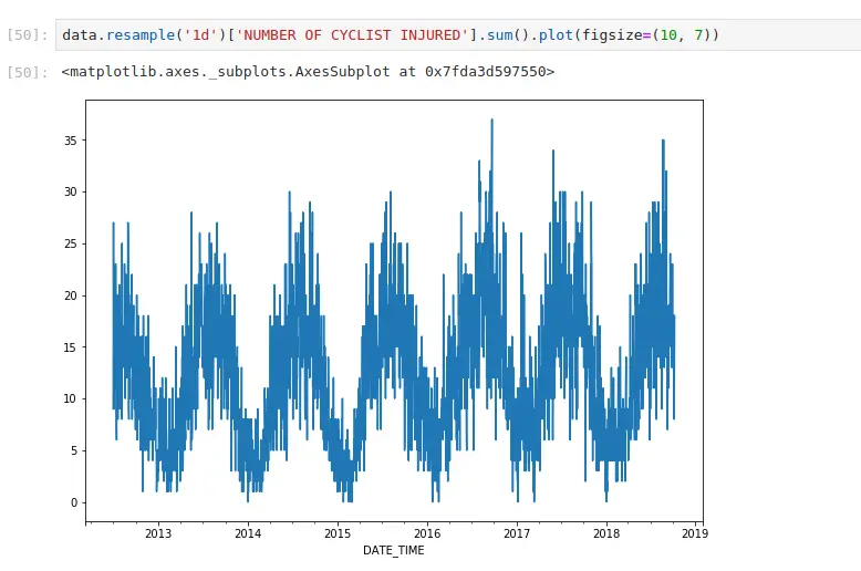
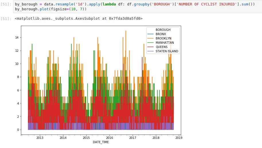
If you’ve ever done groupby operations, resampling works in the same way. It just has nice conventions around time that are convenient. Here, I’m aggregating all cycling injuries by day. I can also apply more complex functions. If I want to generate the same plot, but do it by borough:
One of the subtle things everyone who works with timestamps should be aware of is how pandas will label the result. From the documentation:
Which bin edge label to label bucket with. The default is ‘left’ for all frequency offsets except for ‘M’, ‘A’, ‘Q’, ‘BM’, ‘BA’, ‘BQ’, and ‘W’ which all have a default of ‘right’.
So longer horizon buckets are labeled at the end(right) of the bucket
data.resample('M')['NUMBER OF CYCLIST INJURED'].sum().tail()

#> DATE_TIME 2018-06-30 528 2018-07-31 561 2018-08-31 621 2018-09-30 533 2018-10-31 117
#> Freq: M, Name: NUMBER OF CYCLIST INJURED, dtype: int64
However shorter horizon buckets (including days) are labeled at the start(left) of the bucket
data.resample('h')['NUMBER OF CYCLIST INJURED'].sum().tail()

#> DATE_TIME 2018-10-08 19:00:00 0 2018-10-08 20:00:00 0 2018-10-08 21:00:00 2 2018-10-08 22:00:00 1 2018-10-08 23:00:00 1
#> Freq: H, Name: NUMBER OF CYCLIST INJURED, dtype: int64
This is really important to be aware of — because that means if you’re doing any time-based simulations on aggregations of data (I’m looking at you, FINANCE), and you’re not careful about your labels, you could end up with lookahead bias in your simulation
Rolling Window Operations
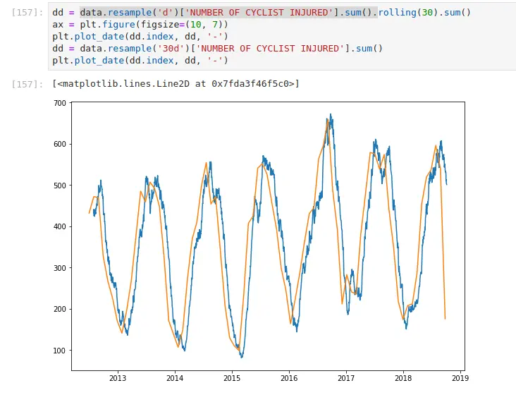
In this example, I take the daily aggregations of cyclists injured in
NYC, and I apply a 30-day moving sum. I also demonstrate what happens if
you resample it to 30 days. A few things become apparent — the label
is still on the left (even though it’s a longer aggregation, it’s based
on 1d so as a result, the label is on the
left) – The data is sparser (since it ticks every 30 d)
The moving average case updates every day, aggregating the past 30 days. Looking at the tail of the data makes it more apparent.
data.resample('d')['NUMBER OF CYCLIST INJURED'].sum().rolling(30).sum().tail()

#> DATE_TIME
#> 2018-10-04    510.0
#> 2018-10-05    513.0
#> 2018-10-06    504.0
#> 2018-10-07    502.0
#> 2018-10-08    501.0
#> Freq: D, Name: NUMBER OF CYCLIST INJURED, dtype: float64
data.resample('30d')['NUMBER OF CYCLIST INJURED'].sum().tail()

#> DATE_TIME
#> 2018-05-31 00:05:00    519
#> 2018-06-30 00:05:00    537
#> 2018-07-30 00:05:00    596
#> 2018-08-29 00:05:00    540
#> 2018-09-28 00:05:00    176
#> Name: NUMBER OF CYCLIST INJURED, dtype: int64
As you can see when we resample by 30d we have
a record every 30 days. In the first case, we have a record every day
(which is an aggregation of the past 30 days)
DateTime Fields
pandas makes it super easy to do some crude seasonality analysis using the DateTime accessors.
Any DateTime column has a dt attribute, which
allows you to extract extra DateTime oriented data. if the index is a
DatetimeIndex, you can access the same fields without the dt accessor.
For example, instead of resampling by d, I could group by the date.
data.groupby(data.index.date)['NUMBER OF CYCLIST INJURED'].sum()
data.groupby(data['DATE_TIME'].dt.date)['NUMBER OF CYCLIST INJURED'].sum().plot()
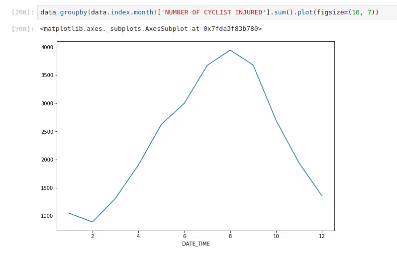
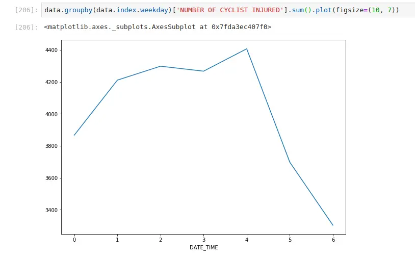
But this means you can get tons of insights by grouping by these fields:
Most injuries happen in the evening commute
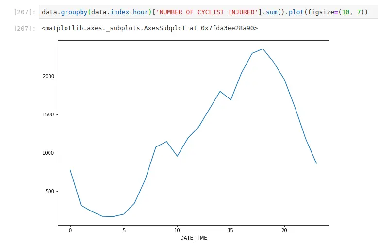
Most injuries happen when it’s warm (when most people cycle)
Fewer injuries occur on the weekend
The Future
This article focuses purely on pandas. As data sizes grow, more and more folks are moving their work to Dask dataframes (multi-node), RAPIDS dataframes (gpu dataframes), and of course, if you put the 2 together, dask-cudf (multi-node, multi-gpu).
The good news is that Dask and RAPIDS actively focus on maintaining API compatibility with pandas where possible. Thanks for reading! Hopefully, this article will save you some time in future jaunts with pandas Timestamps.
At Saturn Cloud, we built a data science platform that lets you use Jupyter, Dask, RAPIDS, and Prefect for everything from exploratory data analysis, ETL, machine learning, and deployment. Try it out for free here.
If you’re an individual, team, or enterprise, there’s a plan that will work for you.
Additional Resources:
- An Intro to Data Science Platforms
- What are Data Science Platforms
- Most Data Science Platforms are a Bad Idea
- Top 10 Data Science Platforms And Their Customer Reviews 2022
- Saturn Cloud: An Alternative to SageMaker
- PDF Saturn Cloud vs Amazon Sagemaker
- Configuring Sagemaker
- Top Computational Biology Platforms
- Top 10 ML Platforms
- What is dask and how does it work?
- Setting up JupyterHub
- Setting up JupyterHub Securely on AWS
- Setting up HTTPS and SSL for JupyterHub
- Using JupyterHub with a Private Container Registry
- Setting up JupyterHub with Single Sign-on (SSO) on AWS
- List: How to Setup Jupyter Notebooks on EC2
- List: How to Set Up JupyterHub on AWS
SHARE:


About Saturn Cloud
Saturn Cloud is your all-in-one solution for data science & ML development, deployment, and data pipelines in the cloud. Spin up a notebook with 4TB of RAM, add a GPU, connect to a distributed cluster of workers, and more. Request a demo today to learn more.
